Comparison of adaptive optical scanning holography based on new evaluation methods

Total view of the OSH system and AOSH system

Previous to introducing the AOSH system, it’s obligatory to offer a concise overview of the OSH system. As a complete rationalization of OSH could be present in quite a few present literature^6,16,17solely a succinct elucidation of the OSH precept will likely be introduced. The experimental configuration of OSH is depicted in Fig. 1. The emitted laser of wavelength (lambda =532 , textnm ) is cut up into two by beam splitter BS1. The temporal frequencies of two beams are modulated into ( omega _0mathrm + Omega ) and ( omega _0 ) by acoustic-optic modulator1 (AOM1) and acoustic-optic modulator2 (AOM2) , respectively. Thus, the heterodyne frequency (Omega ) between these two beams is launched. The higher beam is first collimated by beam expander2 (BE2) after which supplies a spherical wave on object (I_0 (x,y;z)) via the focusing motion by lens1 (L1). The opposite beam is collimated by beam expander1 (BE1); therefore a aircraft wave is projected onto the item. The spherical wave and aircraft wave are mixed by beam splitter2 (BS2), producing a heterodyne interference sample on the scanning mirror. The interference sample is named a time-dependent Fresnel zone plate (TD-FZP)⁷. The TD-FZP oscillates at ( Omega ). The scanning of the item is completed by the scanning mirror, which may scan the 3D object uniformly in a row-by-row method. The scattered mild transmitted via the item is converged to photodetector1 (PD1) by lens2 (L2). The PD1 collects the sunshine and sends {the electrical} sign containing the holographic info of the scanned object to the bandpass filter (BPF) which tunes to {the electrical} sign at frequency ( Omega ). Subsequent, the sign from BPF goes into the lock-in amplifier. Within the meantime, photodetector2 (PD2) delivers a heterodyne sign right into a Lock-in amplifier as a reference sign. Lastly, a posh hologram could be obtained by combining the in-phase output and the quadrature output of the lock-in amplifier. The in-phase and the quadrature-phase outputs of the lock-in amplifier give a sine hologram ( H_sin (x,y) )and cosine hologram ( H_cos (x,y) ) as follows⁷:

and

the place (I_0 (x,y;z)) denotes the depth distribution of the 3-D object, (lambda ) is the wavelength of sunshine in free area, and * denotes 2-D convolution involving x and y⁶.

In accordance with Eqs. (1) and (2), the ensuing complicated hologram H(x, y) within the pc could be expressed as

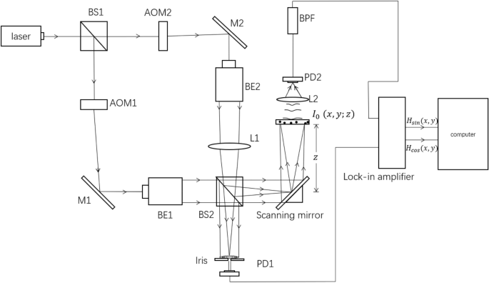
The setup of OSH to file the hologram of object (I_0 (x,y;z)). BS1,2 beam splitter, AOM1,2 acoustic-optic modulator, M1,2 mirrors, BE1,2 Beam expander, L1,2 lens, PD1,2 photodetector.

Within the OSH configuration, the hologram pixels are obtained sequentially in a line-by-line method from the lock-in amplifier, synchronized with the motion of the TD-FZP. The AOSH technique introduces a variety mechanism for the hologram strains, using an error analysis strategy to estimate the extent of “smoothness” between a pair of hologram strains. This analysis facilitates the identification and omission of redundant info inside the hologram strains. The scanning mechanism of AOSH is illustrated in Fig. 2. The important thing facet of the approach lies in the truth that AOSH adjusts the hole between hologram strains by calculating the error analysis.

Idea of the AOSH scanning mechanism¹⁷.

The idea of AOSH is defined as follows. We denote the place of rows that will likely be scanned with the sequence (S = s(j)_0 le j < r )the place j is the index of S, s(j) is the place of the jth scan row, and r is the full scan rows. The expression of the hologram line positioned in s(j) is H(x, s(j)) , and its earlier row and subsequent row is ( H(x,s(j-1)) )and ( H(x,s(j+1)) )respectively. The separation between the hologram line at s(j) and the hologram line at ( s(j-1) ) and ( s(j+1) ) is denoted as (Delta _j – 1) and (Delta _j)respectively. Initially, H(x, s(0)) and H(x, s(1)) must be acquired. Suppose the present scanning hologram line is H(x, s(j)), and the earlier hologram line is (H(x,s(j-1))) saved within the buffer. In AOSH, We calculate the error analysis between the (H(x,s(j-1))) and H(x, s(j)), which may mirror the “smoothness” of a pair of hologram strains, to foretell the place of the following scan row (s(j+1)). The predictor estimates (Delta _j)which is essentially the most important facet of AOSH, at all times want the error analysis to measure the similarity between the earlier hologram line and the present hologram line. Because the error analysis between (H(x,s(j-1))) and H(x, s(j)) is smaller, the hole between s(j) and ( s(j+1) ) turns into wider. The separation between the present and the following scan row is set by the Predictor as

the place ( NEE_j ) denotes the normalized error analysis of jth scan row, which vary is 0 to 1, (Delta _s) and (Delta _MIN) are the components which determine the scanning pace and the hologram high quality. The following place of scan row is expressed as

It may be seen {that a} small ( NEE_j ) ends in giant (Delta _j)and the separation between the present scan row and the following scan row turns into wider. The steps are iteratively carried out till the ultimate row of the item scene has been scanned. After capturing all of the hologram strains, the areas between adjoining hologram strains are crammed with bi-linear interpolation as proven in Fig. 3. Given 2 adjoining hologram strains H(x, s(j)) and (H(x,s(j+1)))the lacking hologram line H(x, m) at vertical place ‘m’ (the place (s(j)< m < s(j + 1))) between them is set as

the place a and b denote the vertical distance between H(x, m) and H(x, s(j)) and H(x, m) and (H(x,s(j+1)))respectively. The time period (fracba + b) and (fracaa + b) are the burden components, which symbolize the contribution of H(x, s(j)) and (H(x,s(j+1))) to H(x, m), respectively.

Filling a row of pixels between a pair of hologram strains.

NRMSE and NMSE in AOSH

Within the previous part, we’ve mentioned the utilization of normalized error analysis (NEE) in AOSH, as depicted in Fig. 2. It’s value noting that the reference 17 introduces AOSH for the primary time¹⁷ by using Normalized-Imply-Error (NME) as a particular NEE technique. NME is the normalized Imply-Absolute-Error(MAE) and owns the identical traits as MAE. Nonetheless, it has been recommended that Root-Imply-Sq.-Error (RMSE) displays superior efficiency to MAE within the analysis of fashions. MAE is affected by numerous common error values, and can’t absolutely mirror some giant errors in contrast with RMSE¹⁹. Contemplating this, we hypothesize that normalized Root-Imply-Sq. Error (NRMSE) might exhibit superior efficiency inside the AOSH framework. Moreover, Imply-Sq. Error (MSE) represents one other generally used error analysis technique, capturing the quadratic nature of errors and offering detailed insights into error evaluation outcomes. Moreover, Normalized Imply-Sq. Error (NMSE) serves as a normalized variant of MSE. Each NRMSE and NMSE current various approaches to normalized error analysis (NEE) inside the AOSH context. On this part, we’ll introduce the precise formulations of those two error analysis strategies in AOSH and elucidate their significance. To facilitate readability, we’ll refer NRMSE-based AOSH as NRMSE-AOSH, NMSE-based AOSH as NMSE-AOSH, and NME-based AOSH as NME-AOSH.

Within the following equations, we denote H(x, s(j)) as the present hologram line; (H(x,s(j-1))) is the earlier hologram line which has been saved within the buffer. x represents the coordinate place of the pixel on the hologram line, and X is the full variety of pixels on the hologram line. (NMSE_j) and (NRMSE_j) denote the NMSE and NRMSE between the ((j-1)^th) and ((j)^th) scan row.

The NMSE and NRMSE in AOSH could be respectively expressed as

and the NME which is the unique technique within the AOSH could be expressed as⁹

The NMSE and NRMSE ,which each are bounded inside the vary [0,1]compute the typical distinction between correspondence pixels between 2 consecutive rows of hologram pixels. Nevertheless, the 2 strategies don’t consider the error in the identical method. As a result of NMSE squares the distinction between pairs of hologram strains, it is going to give extra penalties to the errors between hologram strains. In different phrases, NMSE-AOSH is less complicated to look at the smoothness between holograms, which is able to assist AOSH to skip some comparable info extra adaptively. As an example, for a similar group of holographic line pairs, if a pair of hologram strains corresponding pixels change easily, the place the typical absolute error is lower than one ((frac1Xsum nolimits _mathrmx = 0^{Xmathrm – 1} H(x,s(j)) – H(x,s(j – 1)) < 1)), the worth of (NMSE_j) is smaller than that of (NME_j) as a result of the typical absolute error is squared, which signifies that (Delta _j) calculated by NMSE is bigger than that calculated by NME, as proven in Eq. (2). In different phrases, the smoothness between the hologram line pairs could be amplified by NMSE, and the AOSH scanned strains will likely be lowered. The NRMSE, derived from the sq. root of NMSE, shares an identical attribute with NMSE and is adept at detecting delicate variations inside the information. Due to this fact, NRMSE-AOSH can even present an enhancement to the AOSH system.